The name’s Code. Introducing code.

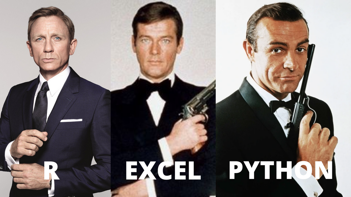
Exploring the lyrics of Bond themes as a way of exploring code with journalists

I’ve been prepping lectures, in particular, a lift-and-dust of my ‘gentle introduction to code’ lecture that I do with my MA Multimedia Journalism students. The aim is not to make them coders, but to introduce them to the concept of coding and how it can help automate the everyday. A good example of that is how code can help us work through mountains of data.

Whilst looking for some suitable data, Billy Ailish ‘dropped’ (which is how I believe we have to say ‘released’ these days) the latest Bond theme. Obviously, there’s a lot of speculation about what it reveals about the film and a lot of analysis about the song itself. This includes a delightfully detailed musical deconstruction by ClassicFM who like the way an “alternating IV and V chords sets up a chorus grounding the harmony of the verse with plenty of harmonic ambiguity.” Metro was one of a number of publications who took the release as an opportunity for a listicle, covering all the Bond film theme tunes.

So I thought having a dig through some data around Bond themes would be an interesting subject to ease students into some code. **

Getting some data

To start with I looked up a list of Bond themes on Wikipedia which is always good for a bit of contextual data. In this case — chart positions etc. Scraping that data into a spreadsheet is pretty easy to do using Google Sheets and its =importHTML()formula.

=importHTML(“https://en.wikipedia.org/wiki/James_Bond_music#Title_themes","Table",2)

I also scraped in the chart positions for each song. The Wikipedia page has them in but there were some gaps and whilst double-checking them, I discovered a post from the Offical Chart Company with “Every James Bond theme ever and where they charted”. I thought they might be a bit more reliable, so I scrapped that into Google Sheets too.

=IMPORTHTML(“https://www.officialcharts.com/chart-news/every-james-bond-theme-ever-and-where-they-charted__10670/","table",1)

With a bit of cut-and-paste and some cleaning up with find and replace and the trim() function to get rid of some pesky spaces and line breaks (\n) at the end of the film titles, I had the workable basic data set with a little bit of context shown below.

Getting Lyrics

The next thing I wanted to do was get the lyrics for each of the songs. There’s plenty of places online to get lyrics for songs and, we’re only talking 24 songs,  so some searching and cut-and-paste wouldn’t be too onerous. But I ended up using Genius.com, partly because I knew it had an API (application program interface) and I could experiment with a bit of code to download lyrics programmatically.

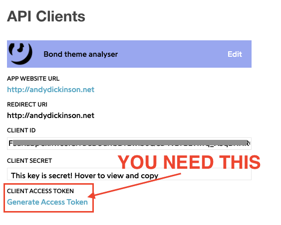
To get access to the API you need to sign up at https://genius.com/api-clients. Then it’s pretty straightforward. You need to define an API client (a defined use of the API). If you want to try the code yourself, you’ll also need to generate an ‘access token’ to use later in the code (if you want to try it yourself that is)

Python and Genius.com

I’ve decided to use Python for this exercise because, well, reasons (see below***). I’ll run through the code here, but there’s also a Google Collabatory version of this post that lets you interact with the code. You’ll get a more detailed idea of what’s going on when the code runs there.

I started with a Python library called lyricsgenius made by John W. Miller. It boils down the Genius.com API into a few easy to use functions. For example, I can search for a song using something like:

song = genius.search_song(songname, artistname)

I’m also using a library called Pandas. It’s designed to work with structured data like CSV files. Using Pandas means I can search, edit, add and delete data like I would in a spreadsheet.

So, a little bit of GiantCap coding and I had a basic Python script that would take my spreadsheet, pull in the song name and artist and then drag in the lyrics. Again, you can see the code run in a more step-by-step way in the Google Collabatory Notebook which I’ll also update through the series.

#Import all the libraries that will help us do the task

import pandas as pd
import re
import os
import lyricsgenius

#The lyricgenius lib needs an access token to work 
genius = lyricsgenius.Genius("<this is where you'd put your access token>")

#Load in the spreashsheet with the basic data
bond_df = pd.read_csv('basic_bond.csv')

#create a temprary store for the lyrics
lyrics =[]

#Work through each row of the spreadsheet and get the artist and the song title and then search Genius with that information and get the lyrics.
for song in bond_df.itertuples():
      print(song[4],song[5])
      song = genius.search_song(song[4], song[5])
      x = song.lyrics
      words = re.sub("[\(\[].*?[\)\]]", "", x)
      words = words.strip()
      words = os.linesep.join([s for s in words.splitlines() if s])
      lyrics.append(words)

#create a new column called 'lyrics' and save all our search results in to that 
bond_df['lyrics'] = lyrics

#Save the output to a new CSV file called bondwithlyrics.csv 
bond_df.to_csv('bondwithlyrics.csv')

It’s worth noting that this isn’t the only way to grab lyrics from Genius. Scraping lyrics for analysis is a popular thing to do and there are loads of interesting variations on the theme that you can find searching ‘Scraping lyrics from genius.com python’.

The code above gave me the following csv file. You can see a new column called lyrics has been added at the end with all of our words.

If you have a quick look through the file you’ll see that Dr No is still causing us problems (the metal hands I guess). We’ve got the lyrics to “A La Nanita Nana” - A Spanish lullaby. The reason for this is that Pandas replaces empty cells with the value Nan or ‘not a number’. When the script searched genius.com it used nan as the search term! We’ll need to remember that the lyrics for Dr No are ‘wrong’ for later.

How ‘long’ is a Bond song?

Looking at the lyrics that I scraped from Genius, I noticed that some songs had more words than others. So I thought it would be fun to compare them. To do that, I needed a quick way to count all the words and then compare them.

The following code does that. It uses pandas again to store the content of the csv file in a temporary object called bond_df We can then tweak and play with the data. In this case, we can count the number of words in each song and save that as a number.

# Load the csv with lyrics into a dataframe
bond_df = pd.read_csv('bondwithlyrics.csv')

# Take the lyrics from each song and split them up when you find a space. 
# Count up the number of words and put that into a new column called 'wordcount'.

bond_df['wordcount'] = bond_df.lyrics.apply(lambda x: len(str(x).split(' ')))

It’s a rough and ready approach, but it does mean I can ask some quick questions. For example, which one had the most words…

#Show me the row in my data that equals the highest valuebond_df.nlargest(1,'wordcount')

The result is Sam Smith’s 2015 ‘Writing’s on the wall’ with 255 words. The shortest…

#Show me the row in my data that equals the highest valuebond_df.nsmallest(1,'wordcount')

We get a weird one here. The shortest in my data is actually Dr No, which, as we know is actually the Spanish lullaby. So I need to expand my search a bit…

#Show me the 5 lowest wordcounts
bond_df.nsmallest(5,'wordcount')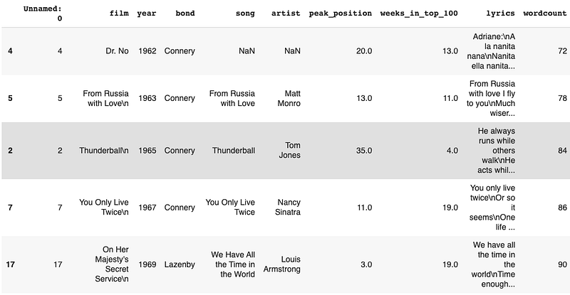

That list shows Matt Munro’s ‘From Russia with love’ has the least lyrics at 78. I also noticed that all of the lowest wordcounts came from early Bond films. It made me wonder if the songs got longer over time — from the 78 of From Russia with love to the 255 of Writing’s on the wall. A quick chart should tell us that…

# Import a library for making charts.
import matplotlib.pyplot as plt

#Plot a scatter chart to show wordcount against year 

bond_df.plot(kind='scatter',x='year',y='wordcount')

The resulting chart, suggests a trend towards longer songs — in wordcount at least.

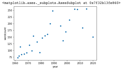
Here’s the same plot with a trend line added to show that trend. I’ve pulled in another library here called Seaborn, which adds some extra visualisation functionality including showing the relationship between the wordcount and year.

import seaborn as sns

#Plot the wordcount against year and show the relationship between the two

sns.regplot(y="year", x="wordcount", data=bond_df);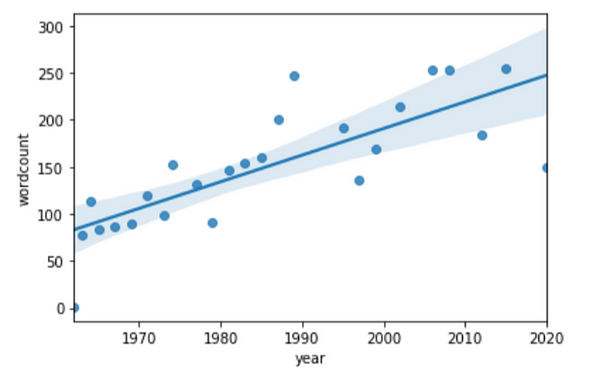

As I thought, a trend towards more lyrics. But does that mean that the songs are getting more complex? Longer? Maybe all pop songs are. Maybe there are more words but they are the same ones. How many times does Shirley Bassey belt out ‘Goldfinger’?

Conclusions

It was surprisingly easy to get a long way down the line with this, just with Google Sheets. What Python did best was to take over on the repetitive stuff — scraping lyrics, counting words etc. And that’s the point. It could be text Bond lyrics to political speeches. Once we have the words in a structured format, coding can help us quickly get to the point where we can start asking questions. I’ve been pretty free with pulling in Libraries to do some of the work for me. That’s, in part down to my magpie-like coding practice. I cut and paste stuff to make it work. In that sense it’s not ‘good code’ but it works.

In the next in this series, I’ll dig a little deeper into lyrics and see what else we can dig up. In the meantime. I hope its whetted your appetite for a bit of code (or a bit of bond)

** In terms of method, this exercise has loads of problems. The choice of Bond themes for example. I’m counting From Russia with Love as the theme to the film of the same name. It wasn’t. The music was, but you only get a hint of Matt crooning over a radio in the early part of the film. So, yes you can drive a bus through the data, but it’s a means to an end.

*** Why Python? I’m a big fan of the Python programming language. It’s one of two that dominate the “journalists that code” and data journalism fields. The other is R. Both are great. You’d benefit from being familiar with both. But I went with Python for this example because a)it’s good for text analysis (yes I know R is too) and I know it well. That’s it really.